9 Measuring and Interpreting Process Performance
A summary can be accurate and still conceal the thing you most need to see.
9.1 Why This Chapter Matters
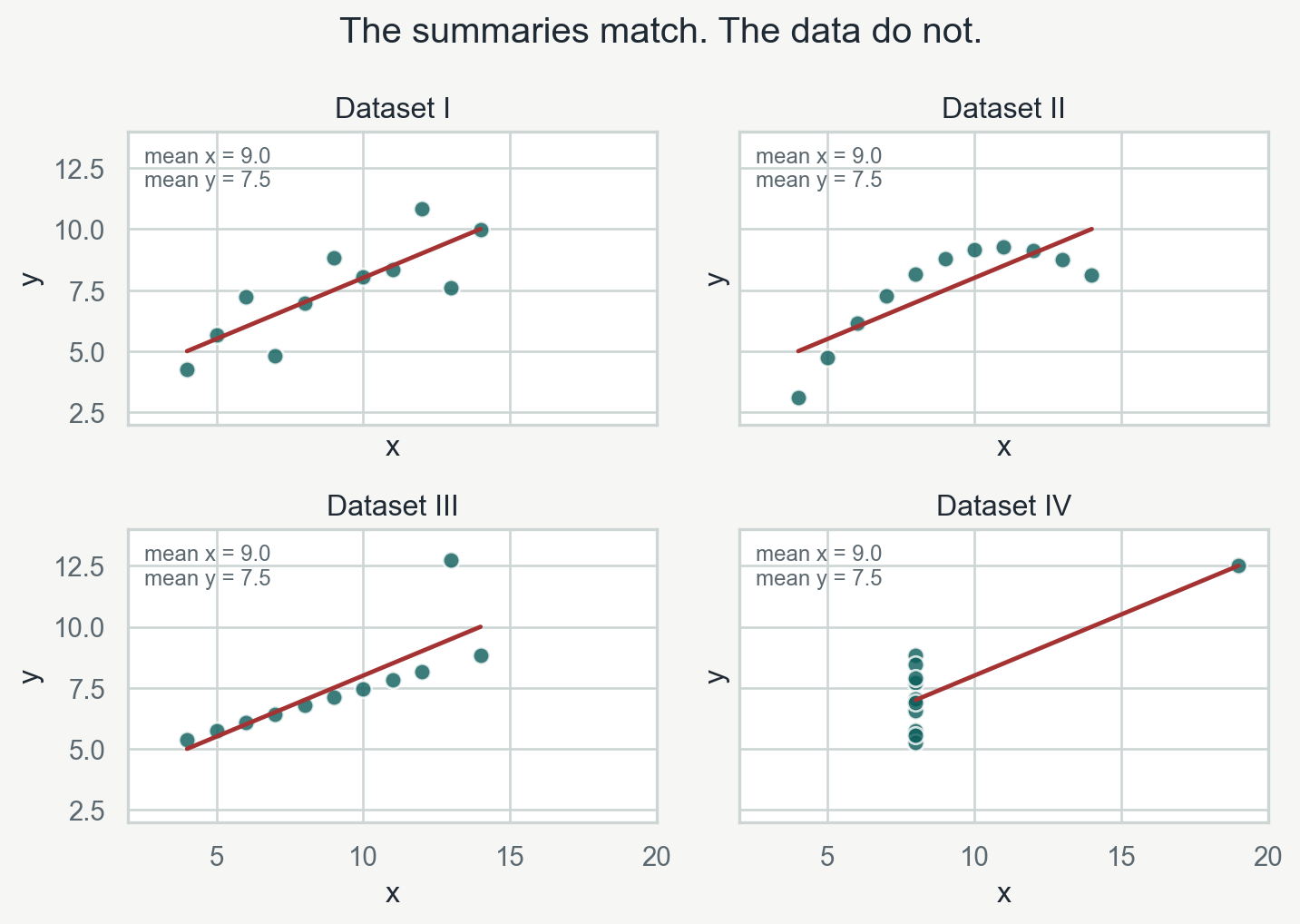
Suppose someone gives you four datasets and reports the following facts about each one:
- the mean of \(x\) is 9.0,
- the mean of \(y\) is 7.5, and
- the same straight line describes the average relationship between \(x\) and \(y\).
Would you expect the observations to look alike?
They do not. One dataset follows the line reasonably well, one bends, one is disrupted by an unusual observation, and one depends almost entirely on a single distant point. These are Anscombe’s quartet, constructed to demonstrate why numerical summaries should be inspected alongside the observations they summarize (Anscombe 1973).
The lesson is not that averages are bad. The lesson is that every summary answers a limited question. Before trusting one, we need to know what was observed, how the observations are distributed, and what decision the summary is supposed to support.
Wash n’ Fold now presents the same problem in operational form. The event log contains hundreds of timestamps, the map displays a few averages, and customers experience individual orders rather than averages. This chapter turns those records into a baseline we can inspect and use.
9.2 Learning Objectives
By the end of this chapter, the student will be able to:
- Data Understanding Explain how a distribution describes the observed values of a quantity and how often or where those values occur Bloom:Understand
- Data Understanding Aggregate an event log into activity and order summaries using count, sum, minimum, maximum, range, mean, median, and mode while preserving units and the group being summarized Bloom:Apply
- Statistical Analysis Calculate and interpret takt time, processing time, cycle time, operating lead time, and PCE using consistent boundaries and explicit treatment of rework Bloom:Apply
- Statistical Analysis Interpret tabular and graphical evidence to compare typical, tail, and threshold performance using mean, median, nearest-rank percentiles, and the customer-promise violation rate Bloom:Analyze
- Statistical Analysis Use WIP, throughput, and Little’s Law with a matching boundary and observation period, distinguishing average WIP from a snapshot Bloom:Apply
- Lean Six Sigma Principles and Tools Connect a Wash n’ Fold metric symptom to a first-pass waste hypothesis and the evidence needed to test it Bloom:Analyze
9.3 From Events to Customer Observations
Chapter 7 introduced the event log as the foundational record. Chapter 8 calculated each activity record’s P/T, W/T, and S/T, grouped comparable records on the Mapping Worksheet Set, and transferred selected averages to the current-state map. That compression made the flow readable, but it also hid the individual observations.
Now we return to them. We need to know how the process behaved across complete customer orders, whether the average represents most customers reasonably well, and which evidence should direct the next investigation. All calculations in this chapter can be done on paper, with a basic calculator if useful. The charts help you inspect the evidence; you are not expected to create them at White Belt.
| Artifact | Question it answers | What one row represents |
|---|---|---|
| Event log | What happened? | One order- or load-level activity record linked to its parent case |
| Map worksheet | What does each activity look like across observations? | One activity with counts and timing summaries |
| Process map | How does work move and where does it wait? | Selected activities, queues, and paths |
| Order summary | What happened to this customer’s order? | One complete order |
| Performance readout | How did a defined group of orders perform? | A metric with its group, units, and period |
These artifacts do not compete. The log preserves individual events, the worksheet supports the map, the order summary reconstructs each customer’s experience, and the performance readout brings those measures together so we can decide what to investigate.
NoteEvidence and Clock
We continue with current-state Friday 91 from Chapter 8: 39 orders, including 21 dropped off by 9:00 a.m. One customer order is the unit of analysis; its boundary runs from drop-off through staging and readiness notification. Pickup and payment remain outside it.
Minute 0.0 is 7:00 a.m.; minute 120 is 9:00 a.m.; minute 600 is the 5:00 p.m. promise; minute 690 is the 6:30 p.m. close. The model follows unfinished orders on a cumulative operating-time clock until all are ready. Closed hours are omitted. These are operating lead times, not overnight calendar durations.
- Download the activity event log
- Download the aggregated activity worksheet data
- Download the learner order summary
Keep your Chapter 8 map and Participant Verification Record beside these tables. For a first complete-order check, use WNF-003: its nine activity records include two compatible Wash loads, two Dry loads, and one Fold correction. Read its timestamps in the source excerpt, compare them with the worked timing sheet, and then locate its single row in the learner order summary. Its drop-off-to-readiness operating lead time is 166.3 minutes, rather than the sum of every child-load duration.
The order summary derives its durations from the displayed one-decimal event-log timestamps. This keeps the hand calculations reproducible.
9.4 What Are We Actually Summarizing?
Aggregation means combining observations into a summary. Before calculating, complete this sentence:
This number describes ___ for , measured in , across ___.
For example, “30.4 minutes” is incomplete. “Mean Wash P/T was 30.4 minutes per load across 65 observed loads” identifies the quantity, aggregation, physical unit, observation unit, and group. It is still not the duration of one particular load.
The same log supports several groupings: by load for machine activity, by activity for mapping, and by order for customer lead time. A sum of all event-log rows is not automatically the elapsed time of one order or the shop’s working day.
9.4.1 A Distribution Is the Pattern of Observations
Take the five L1 Wash P/T observations selected for Chapter 8’s short practice excerpt, WNF-001 through WNF-005, in minutes:
\[ 35.0,\ 32.7,\ 30.0,\ 29.4,\ 26.3 \]
These five values form an observed distribution. A distribution describes which values were observed and how often or where those values occur. With five values, we can inspect every observation directly. With 65 loads or hundreds of customer orders, a graph often makes the shape, gaps, clusters, and unusual values easier to see than a long table does.
Exploratory data analysis begins with that act of inspection. We look before deciding which summaries are adequate, which comparisons are fair, or which observations deserve another question.
9.4.2 Count, Sum, and Mean
Count tells us how many observations there are: \(n = 5\). Sum adds their values: \(35.0 + 32.7 + 30.0 + 29.4 + 26.3 = 153.4\) minutes. Mean, or arithmetic average, divides the sum by the count:
\[ \begin{aligned} \mathrm{Mean} &= \frac{\text{Sum}}{\text{Count}} \\ &= \frac{153.4}{5} \\ &= 30.68 \approx 30.7\text{ minutes} \end{aligned} \]
The sum is the total of five load-level processing durations. It is not 153.4 minutes on one washer’s clock: the loads belong to different orders and may occupy different machines in parallel. For the full 65-load Wash group, the P/T sum is 1,977.2 minutes, giving a mean of \(1,977.2/65 \approx 30.4\) minutes.
Use the mean when the total burden is meaningfully distributed across the observations: average work per load, average lead time per order, or average demand per day. Do not ask it to show the shape of the distribution or the experience of every customer.
9.4.3 Minimum, Maximum, and Range
Sort those five observations:
\[ 26.3,\ 29.4,\ 30.0,\ 32.7,\ 35.0 \]
The minimum is 26.3 and the maximum is 35.0. They describe the shortest and longest observed durations; they are not guaranteed operating limits. Their difference, \(35.0 - 26.3 = 8.7\) minutes, is the observed range.
The range answers a practical first question: how far apart were the shortest and longest observations? Because it depends only on those two observations, one extreme value can change it sharply.
9.4.4 Median and Percentiles
The median is the middle sorted observation: 30.0 minutes. With an even count, average the two middle observations. For example, the median of \(26.3, 29.4, 30.0, 32.7\) is \((29.4 + 30.0)/2 = 29.7\).
The mean uses every value, so one very long record can pull it upward. The median describes the middle position. Neither describes every customer’s experience.
A percentile is also a position in a sorted distribution. The 25th percentile, or P25, marks the lower quarter; P50 is the median; P75 marks the upper quarter; and P90 marks the slow tail used later in this chapter.
The conventional five-number summary is:
- minimum,
- first quartile, \(Q_1\) or P25,
- median, or P50,
- third quartile, \(Q_3\) or P75, and
- maximum.
It gives a compact account of position and spread. It does not include the mean, count, or sum, and it does not replace inspection of the observations. Software uses several percentile conventions, so record the convention when the choice can change the reported value.
9.4.5 Mode and Frequency
The mode is the value or category occurring most often. In the representative Friday, 13 orders used one compatible load and 26 used two. The modal load count is therefore two.
This does not mean every order used two loads. The mean load count is \((13 \times 1 + 26 \times 2)/39 \approx 1.67\). That fractional average is useful for planning across many orders, even though no individual order used 1.67 loads.
There is no useful single mode in the five distinct Wash P/T values above. Several values can tie for most frequent, and rounding continuous durations can create ties. Mode is often more informative for counts or categories, such as load count or correction reason, than for precisely timed work.
9.4.6 Keep the Summary Attached to Its Evidence
| Summary | Hand calculation | Question |
|---|---|---|
| Count | Count the relevant rows | How many observations support this? |
| Sum | Add the values | How much across this group? |
| Minimum / maximum / range | Read the ends and subtract minimum from maximum | What extremes and total spread did we observe? |
| Mean | Sum divided by count | What is the average per observation? |
| Median | Find the middle of the sorted list | What is the middle observation? |
| Percentile | Locate a stated position in the sorted list | How did the middle or tail behave? |
| Mode | Tally each value or category | What occurs most often? |
The Mapping Worksheet can preserve the count, sum, and mean needed for the map. The baseline performance readout can add distribution summaries needed for a customer or system question. Both must point back to the observations. Do not treat an empty measurement as zero or average unrelated activities together.
If two groups have different counts, combine their sums and counts before finding the combined mean. For two orders averaging 10 minutes and eight averaging 20 minutes, the combined mean is \((2 \times 10 + 8 \times 20)/10 = 18\) minutes, not 15. The same caution applies to daily promise-violation rates.
ImportantPause and Check
Using the five Wash observations, calculate count, sum, mean, minimum, maximum, range, and median. Then write one complete measurement statement that identifies the aggregation, quantity, physical unit, observation unit, and group.
9.5 From Activity Records to Complete Orders
To build an order row, find its first Drop-off queue entry and its final Stage and notify work end. Subtract the first timestamp from the last. Then group the rows by activity before adding durations across the order. Order-level activities contribute one record each. For Wash and Dry, preserve the separate load records but collapse their parallel timing into the order’s elapsed activity span; never add parallel load durations and call the result customer lead time.
Here are WNF-003’s activity records in time order, so you can reconstruct an order on paper without opening a data file. All timestamps are elapsed operating minutes; each row is pass 1 of its named activity for this order or load.
| Activity | Load ID | Queue entry | Setup start | Work start | Work end |
|---|---|---|---|---|---|
| Drop-off and ticket | — | 12.1 | 13.4 | 13.4 | 16.6 |
| Sort and tag | — | 16.6 | 16.6 | 16.6 | 21.5 |
| Wash | L1 | 21.5 | 23.9 | 25.1 | 55.1 |
| Wash | L2 | 21.5 | 25.1 | 26.3 | 56.3 |
| Dry | L1 | 56.3 | 56.3 | 57.0 | 108.5 |
| Dry | L2 | 56.3 | 57.0 | 57.6 | 109.1 |
| Fold and package | — | 109.1 | 129.1 | 129.6 | 142.5 |
| Fold correction | — | 142.5 | 148.9 | 148.9 | 153.0 |
| Stage and notify | — | 153.0 | 173.7 | 173.7 | 178.4 |
Subtract work start from work end for P/T, queue entry from setup start for W/T, and setup start from work start for S/T. The resulting order summary begins:
| Order | Arrival | Ready / notified | Total P/T | Total W/T | Total S/T | Operating L/T |
|---|---|---|---|---|---|---|
| WNF-001 | 9.1 | 174.3 | 109.8 | 51.2 | 4.2 | 165.2 |
| WNF-002 | 10.9 | 173.7 | 106.9 | 50.4 | 5.5 | 162.8 |
| WNF-003 | 12.1 | 178.4 | 111.3 | 50.8 | 4.2 | 166.3 |
All values are minutes. For WNF-003, \(178.4 - 12.1 = 166.3\), and \(111.3 + 50.8 + 4.2 = 166.3\). Its nine activity records include two Wash loads, two Dry loads, and one Fold correction; the other two displayed orders have eight records because they have no correction.
These equalities work because the order summary first collapses each set of parallel Wash or Dry load records into one order-level elapsed span. Do not add parallel machine durations and call the sum customer elapsed time. For a different process, check that property before using the same shortcut.
Counting the two Y flags at Fold and package and Fold correction would double-count WNF-003’s defect. One flag identifies the trigger and the other identifies correction work. Count the correction record or the distinct affected order, according to the question.
9.5.1 Total Processing Time, Cycle Time, and Lead Time
Definition 9.1
NoteDefinition: Total Processing Time
Total processing time is the sum of the processing times on one unit’s path, including repeated work. Average total processing time averages those unit totals. Active processing includes automatic machine cycles; it does not mean a worker is occupied throughout.
Definition 9.2
NoteDefinition: Cycle Time
Cycle time, written C/T, is the observed time between successive completions from a process or process step. For repeating operator work, it can also describe the time required to complete the work elements before the sequence repeats. In a stable, sequential one-piece operation, one unit’s P/T and the C/T between completions may be numerically equal; the labels still answer different questions. Cycle time is a completion pace, not the sum of processing times along a unit’s path.
The timing-terms note in Chapter 8 identifies the Rother and Shook convention used here and the alternate Hopp and Spearman convention. In either convention, identify the start event, stop event, observation unit, aggregation, and physical unit before comparing two reported numbers.
Definition 9.3
NoteDefinition: Lead Time
Lead time, written L/T, is the elapsed time between the defined start and stop events for one work unit. Unless another clock is stated, elapsed lead time includes all calendar time within that boundary.
Definition 9.4
NoteDefinition: Operating Lead Time
Operating lead time counts only the periods in which the process is scheduled to operate between the defined start and stop events. Wash n’ Fold uses drop-off to ready-and-notified and excludes closed hours. Report the operating calendar whenever this measure is used.
For sequential, fully accounted order intervals:
\[ \mathrm{L/T} = \mathrm{P/T} + \mathrm{W/T} + \mathrm{S/T} \]
Here P/T includes all active processing, VA and non-VA; W/T includes all waits; S/T includes preparation before processing. Keep setup separate even when it is small. An absent measurement does not justify dropping the S/T term.
9.5.2 Check the Worksheet Against the Orders
The activity worksheet mixes 65-load Wash and Dry summaries with 39-order summaries for the other activities. Adding those means would mix observation units and cannot produce order lead time.
Instead, collapse each order first and then average the complete order rows. The order summary gives mean P/T of 104.5 minutes, mean W/T of 554.0 minutes, and mean S/T of 4.1 minutes, which add to the 662.6-minute mean operating lead time. Those order-level means already include the observed correction paths.
If you estimate the correction contribution separately, remember that not every order followed that path. Five of the 39 orders each had one correction record averaging 6.8 minutes of work and 5.6 of waiting.
Their average contribution across all orders is:
\[ \frac{5}{39}(6.8 + 5.6) \approx 1.6\text{ minutes per order} \]
Do not add 12.4 minutes to every order or divide correction time by 39 when describing the correction activity itself. The correct denominator depends on the question.
Means can be added when they refer to the same orders and account for how often each path occurs. Adding activity medians or P90s does not give the median or P90 of complete orders. Calculate those from the complete order operating-lead-time list.
9.6 Typical, Tail, and Promise Performance
An average answers one question about the group. A delivery promise asks whether particular orders met a deadline.
The table below contains all 21 orders dropped off by 9:00 a.m. Before reading further, try to identify the shape of their operating-lead-time distribution, the middle order, and the slow tail by scanning the rows. This is possible, but it is harder than it needs to be.
Use it for the promise analysis; the remaining 18 orders are outside that promise cohort. All timestamps are elapsed operating minutes.
| Order suffix | Arrival | Ready / notified | Operating L/T | Missed promise? |
|---|---|---|---|---|
| 001 | 9.1 | 174.3 | 165.2 | N |
| 002 | 10.9 | 173.7 | 162.8 | N |
| 003 | 12.1 | 178.4 | 166.3 | N |
| 004 | 31.8 | 286.3 | 254.5 | N |
| 005 | 33.7 | 286.9 | 253.2 | N |
| 006 | 44.1 | 290.5 | 246.4 | N |
| 007 | 47.8 | 390.9 | 343.1 | N |
| 008 | 52.8 | 391.9 | 339.1 | N |
| 009 | 60.3 | 394.6 | 334.3 | N |
| 010 | 61.2 | 485.7 | 424.5 | N |
| 011 | 62.1 | 485.3 | 423.2 | N |
| 012 | 63.6 | 488.8 | 425.2 | N |
| 013 | 75.3 | 593.4 | 518.1 | N |
| 014 | 78.2 | 589.7 | 511.5 | N |
| 015 | 81.0 | 590.5 | 509.5 | N |
| 016 | 88.0 | 686.3 | 598.3 | Y |
| 017 | 89.7 | 685.7 | 596.0 | Y |
| 018 | 97.4 | 688.8 | 591.4 | Y |
| 019 | 100.0 | 782.0 | 682.0 | Y |
| 020 | 103.1 | 781.5 | 678.4 | Y |
| 021 | 110.5 | 786.7 | 676.2 | Y |
Now inspect the same orders as points arranged from fastest to slowest.
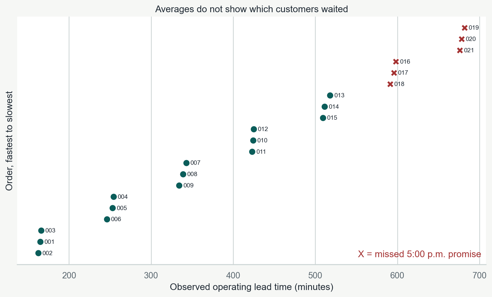
The groups of similar operating lead times, the gaps between them, and the six promise misses are visible without asking the eye to coordinate five table columns. The table remains necessary when we need an exact timestamp or must reproduce a calculation. The plot and table answer different questions about the same evidence.
The 21 operating lead times sum to 8,899.2 minutes, so their mean is \(8,899.2/21 \approx 423.8\) minutes. Sorted, they are:
162.8, 165.2, 166.3, 246.4, 253.2, 254.5, 334.3, 339.1, 343.1, 423.2, 424.5, 425.2, 509.5, 511.5, 518.1, 591.4, 596.0, 598.3, 676.2, 678.4, 682.0.
The minimum is 162.8, the maximum is 682.0, and the range is \(682.0-162.8=519.2\) minutes. Using the nearest-rank convention, \(Q_1\) is the sixth observation, 254.5 minutes; the median is the 11th observation, 424.5 minutes; and \(Q_3\) is the 16th observation, 591.4 minutes.
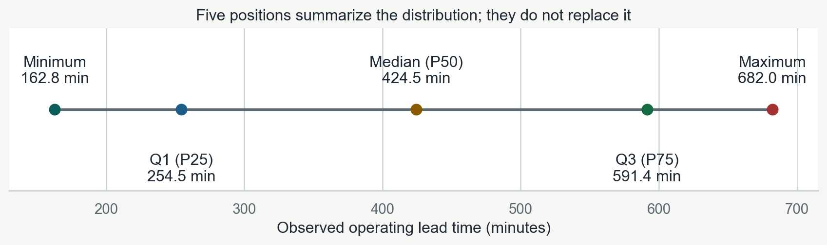
The mean of 423.8 minutes happens to sit near the median, but that agreement does not make the distribution narrow. Half of the observed lead times span more than 336 minutes between \(Q_1\) and \(Q_3\).
9.6.1 Find P90 by Hand
The 90th percentile, or P90, is a way to describe the slow tail. For this chapter, use the nearest-rank rule:
- Sort the observations from smallest to largest.
- Multiply the count by 0.90.
- Round that position upward to a whole number, if necessary.
- Read the observation at that position, counting from one.
For 21 orders, \(0.90 \times 21 = 18.9\), so use position 19. P90 is therefore 676.2 minutes: at least 90% of these observed orders had operating lead times no greater than this value. It is a sample description, not a guarantee about the next order.
An empirical cumulative distribution, or ECDF, plots every observed value against the proportion of observations at or below it. To read a percentile, begin with a proportion on the vertical axis, move to the observed staircase, and then read the corresponding time on the horizontal axis.
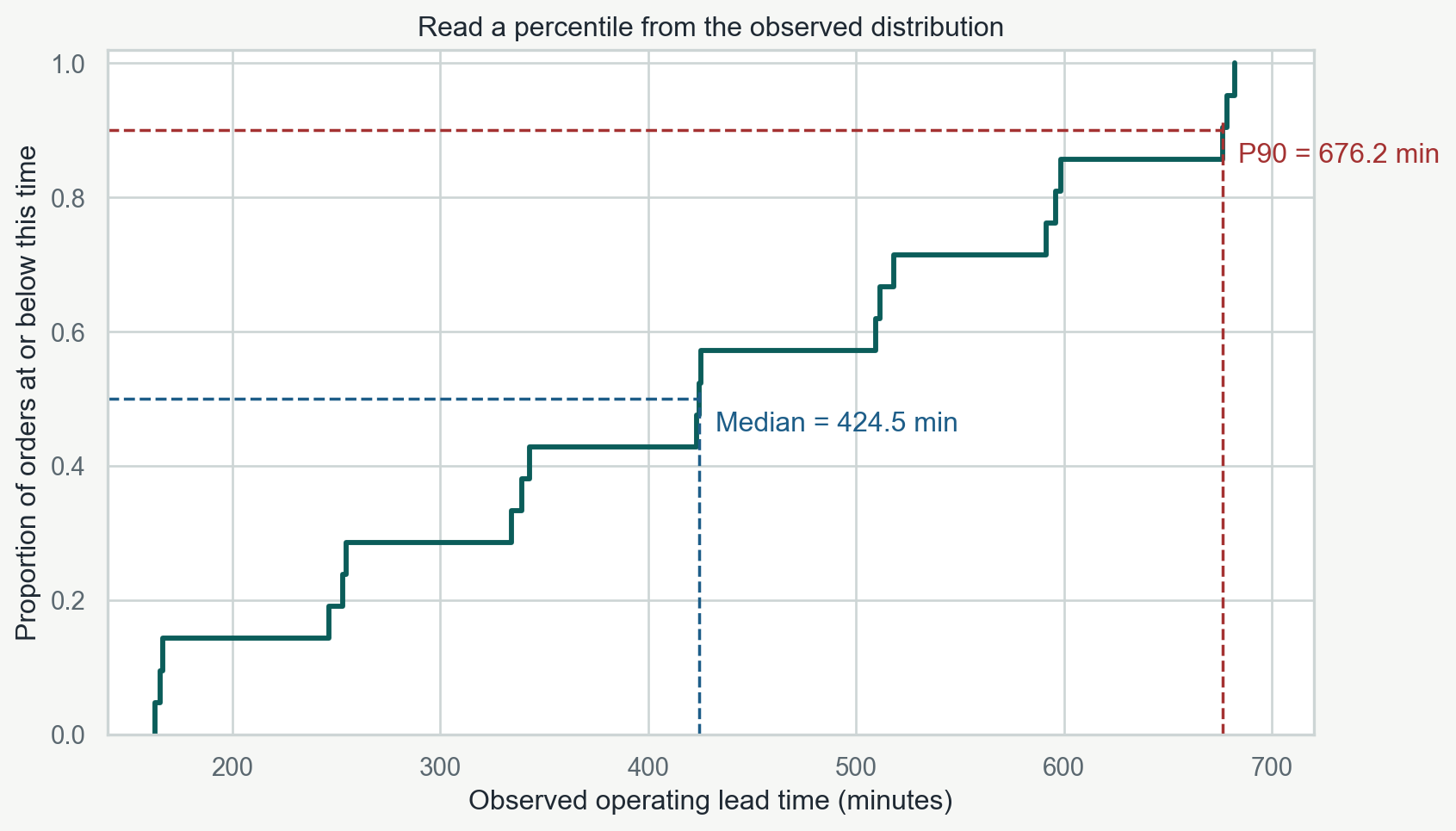
The ECDF preserves all 21 observations while making P50 and P90 visible. Unlike a histogram, it does not require us to choose arbitrary bin widths.
Software offers several percentile conventions, including interpolation between observations. Record which one you use. The technical simulation exports use an interpolated P90; the pencil-and-paper readout here uses nearest rank consistently. A small difference between those results is a method difference, not a change in the orders.
9.6.2 Count Promise Violations
An order is eligible if arrival is at or before minute 120. An eligible order violates the promise if readiness notification is after minute 600. Exactly 5:00 p.m. counts as on time.
Let \(M\) be the number of eligible orders that miss the promise and \(E\) be the total number of eligible orders.
\[ \begin{aligned} \text{Violation rate} &=\frac{M}{E}\times100\% \\ &=\frac{6}{21}\times100\% \\ &\approx28.6\%. \end{aligned} \]
WNF-016 has a lead time of 598.3 minutes, which is below 600, but it still misses the promise. It arrived at minute 88.0 and was ready at 686.3. A fixed clock deadline is different from a fixed allowance measured from arrival.
The mean and P90 describe operating lead times; the violation rate tests the promised deadline. None substitutes for the others.
9.6.3 Keep the Two Cohorts Separate
| Measure | All 39 orders | 21 promise-eligible orders |
|---|---|---|
| Mean operating L/T (min) | 662.6 | 423.8 |
| Median operating L/T (min) | 678.4 | 424.5 |
| Minimum / maximum (min) | 162.8 / 1,152.8 | 162.8 / 682.0 |
| P90, nearest rank (min) | 1,057.8 | 676.2 |
| Promise-violation rate | Not defined for this whole group | 6/21 = 28.6% |
Later arrivals also experience the growing release queue. Including them changes the operating-lead-time summary; it does not change which orders qualify for the 9:00 a.m. promise. The project target remains approximately 28% to 10% within 30 days.
The baseline performance readout should preserve this distinction rather than offering one unlabeled “current average.” For each reported metric, record the quantity, value, unit, aggregation, observation unit, boundary, cohort or period, and any calculation convention that another reader would need to reproduce it.
ImportantCompare Two Questions
Explain why a report of “average operating lead time 423.8 minutes” is incomplete without its cohort. Then explain why dividing the six violations by all 39 orders would misrepresent promise performance.
9.7 Read the Process as a System
The distribution tells us what customers experienced. It does not yet tell us whether the shop can keep pace with demand, where elapsed time accumulates, or how unfinished work relates to completion rate. The next measures answer those system questions.
9.8 Takt Time, Demand, and Capacity
The first system question is whether the process can finish work at the pace customers require. Takt translates demand into that required pace; capacity estimates what the available resources could accomplish; throughput records what the process actually completed.
Definition 9.5
NoteDefinition: Takt Time
Takt time is available production time in a planning period divided by demand for that same period:
\[ T = \frac{A}{D} \]
For planning, use approximately 38 orders per Friday and 690 operating minutes:
\[ T = 690/38 \approx 18.2\text{ minutes per order} \]
Using the simulation’s unrounded average demand of 37.73 gives 18.3 minutes. Using the representative day’s actual 39 orders gives 17.7 minutes. Label whether the calculation uses forecast demand or an observed day’s demand.
The cell has two workers, six washer positions, six dryer positions, and two folding stations. Do not multiply the shop’s 690-minute clock by its employee count for customer Takt. Staff minutes matter separately when estimating labor capacity. The model assumes these resources are available for the stated operating period; in an observed business, scheduled downtime and staffing changes need explicit treatment.
Orders arrive between 7:00 and 11:00, much faster than the whole-day completion pace. The modeled mean interarrival time is 6.4 minutes. Arrival cadence, required average completion pace, and actual throughput are three different measures.
A 45-minute dry cycle does not by itself imply capacity of one order every 45 minutes. Several orders can dry in parallel, and some occupy two positions. A supplied planning estimate using the current modeled work content is:
| Resource | Estimated capacity (orders/hour) |
|---|---|
| Two workers, across all their tasks | 3.56 |
| Six washer positions | 6.28 |
| Six dryer positions | 4.46 |
| Two folding stations | 6.69 |
These estimates use the 100-run current-state work mix and include setup and correction work. For example, approximately 33.7 worker-minutes per order gives \(2 \times 60/33.7 \approx 3.56\) orders/hour. They are resource-workload estimates, not observed completion rates or guaranteed schedules.
The smallest estimate is 3.56 orders/hour. Daily demand averages about 3.28 orders per operating hour, below that physical estimate. This justifies testing whether the release rule leaves usable capacity idle. It does not guarantee that a burst of morning orders will meet a 5:00 p.m. deadline. The log is needed to check what the process actually accomplishes.
9.9 Process Cycle Efficiency
The next question is where the customer’s elapsed time goes. If active work occupies only a small part of lead time, making one active step slightly faster may leave the customer experience almost unchanged.
Definition 9.6
NoteDefinition: Process Cycle Efficiency
Process cycle efficiency, or PCE, is the share of lead time spent in value-added work:
\[ PCE = \frac{\text{Value-added time}}{\text{Lead time}}\times100\% \]
For a group of orders, this book’s White Belt convention is to divide total VA time by total lead time for the same orders. That equals mean VA time divided by mean lead time for that group. It need not equal an unweighted average of individual orders’ PCE percentages. When the study uses an operating clock, name the denominator as operating lead time and use that same clock throughout.
Wash, Dry, and Fold and package supply the VA time in this case. Correction, intake, sorting, staging, waiting, and setup remain outside the numerator.
Across the 39 orders, VA time sums to 3,582.3 minutes and operating lead time sums to 25,840.5 minutes:
\[ PCE = \frac{3,582.3}{25,840.5}\times100\% \approx 13.9\% \]
This says that approximately 13.9% of the summed order operating lead time is classified VA. It is not worker utilization, machine utilization, or a universal quality score. There is no universal “good PCE” threshold in this chapter. Compare like boundaries and ask which non-VA contributions can be reduced without harming quality.
The order-level P/T, W/T, and S/T means reveal the practical consequence more directly.
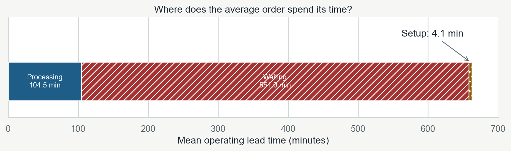
Waiting accounts for 554.0 of the 662.6 mean operating minutes. That does not prove why the orders waited, but it tells the team why shaving a minute from an already short active task is unlikely to solve the customer problem.
9.10 WIP, Throughput, and Little’s Law
The final system question connects unfinished work, completion rate, and elapsed time. This matters because a team can move work out of sight, count it at a convenient instant, or celebrate a busy resource without improving the rate at which complete orders leave the system.
Work in process, or WIP, is unfinished work inside the chosen boundary. Throughput is completions per unit of time. Little’s Law relates averages:
\[ \begin{aligned} \mathrm{Average\ WIP} &= \text{Throughput} \\ &\quad \times \text{Average lead time} \end{aligned} \]
\[ \mathrm{Average\ lead\ time} = \frac{\text{Average WIP}}{\text{Throughput}} \]
Use the same work unit, boundary, and time basis throughout. Average WIP describes how much work is present over the observation period. It is not the number present at one convenient instant.
9.10.1 A Small WIP Calculation
Suppose there are two open orders for 30 minutes and four for the next 30 minutes. Average WIP over that hour is \((2 \times 30 + 4 \times 30)/60 = 3\) orders.
For unequal durations, weight each count by how long it persisted. Two orders for 10 minutes and four for 50 minutes gives \((2 \times 10 + 4 \times 50)/60 \approx 3.67\), not three.
9.10.2 Use the Relationship, Then Check Its Assumptions
Suppose a support process averages 50 open tickets over a representative period and completes 10 tickets per working day:
\[ \begin{aligned} \mathrm{Average\ lead\ time} &= \frac{50\text{ tickets}}{10\text{ tickets/day}} \\ &= 5\text{ working days} \end{aligned} \]
At unchanged throughput, a three-day target corresponds to \(10 \times 3 = 30\) average open tickets. That relationship does not tell us which operational change will achieve it. Simply moving tickets outside the reported boundary would improve the number without improving customer experience. Reducing WIP too far can also starve resources and reduce throughput.
9.10.3 Reconcile the Wash n’ Fold Full Run
The representative run starts empty at minute zero and follows all 39 orders to completion at approximately minute 1,377.6. For this full cohort, the sum of order operating lead times is also the area under the open-order WIP history: 25,840.5 order-minutes.
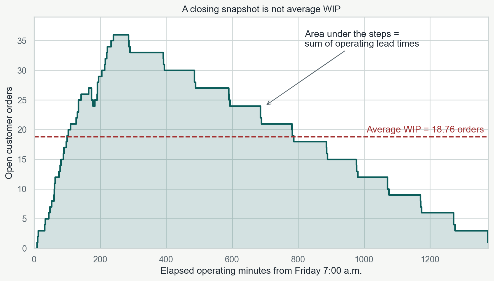
The chart makes the distinction between a snapshot and an average visible. The process has 21 open orders at closing time, but the height of the curve changes throughout the run. Average WIP depends on the whole shaded area, not one selected point. Dividing 25,840.5 order-minutes by the 1,377.6-minute run gives:
\[ \mathrm{Average\ WIP} \approx 18.76\text{ orders} \]
Mean operating lead time is \(662.6/60 \approx 11.04\) operating hours. Little’s Law therefore gives approximately:
\[ \mathrm{Throughput} = \frac{18.76}{11.04} \approx 1.70\text{ orders/hour} \]
The direct count agrees: \(39/(1,377.6/60) \approx 1.70\) orders/hour. This is an accounting check over a complete start-empty/end-empty run, not independent proof of the simulation or a claim that Friday arrivals were steady. For ongoing operations, use a representative period and account for work carried across its boundaries.
At the 6:30 p.m. close, only 18 orders are ready and 21 remain open. That snapshot is useful operationally, but pairing 21 with the full-run mean operating lead time would mix different measures. Likewise, \(18/11.5 \approx 1.57\) orders/hour describes by-close throughput, not full-run throughput.
The capacity estimate of 3.56 orders/hour and the realized full-run rate of 1.70 answer different questions. Their gap supports investigating the serial rule that holds the next wash batch until all orders in the active batch clear drying. Little’s Law relates the observed averages; capacity and release rules help explain why they take those values.
9.11 Build the Baseline Performance Readout
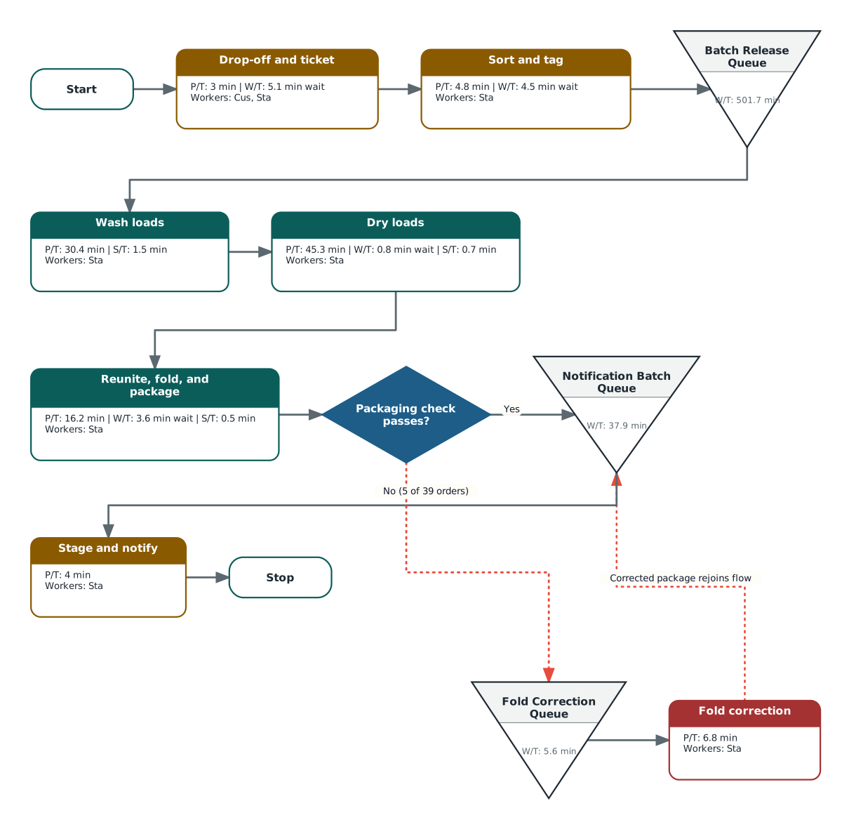
The map shows where work moves and waits. The Baseline Performance Readout records what the selected measures say about the defined process and what the team should inspect next.
For every reported metric, the readout names:
- the quantity and value,
- whether it describes one observation or an aggregate,
- the observation unit and physical unit,
- the process boundary,
- the cohort and observation period, and
- the operational question or next check.
Wash n’ Fold uses the completed readout below as the model. For your capstone, construct the same kind of compact readout from your before-state observations. Use the blank Baseline Performance Readout as a PDF, XLSX, or CSV. The completed Friday 91 version is available as a PDF, XLSX, or CSV. Its separate metric rows keep the value, aggregation, units, boundary, cohort, clock, supported signal, and next question inspectable. The charts in this chapter help you learn to inspect distributions; creating those charts is not a White Belt capstone requirement.
Readout scope: simulated representative Friday 91; drop-off through staging and readiness notification; operating minutes from 7:00 a.m.; one customer order as the case unit. Rows identify whether they use all 39 orders, the 21 promise-eligible orders, or a smaller set of activity records.
| Measure and result | Aggregation and unit | Supported signal | Next question or check |
|---|---|---|---|
| Mean operating L/T 662.6 min; mean W/T 554.0 min | Means across all 39 orders; minutes per order | Waiting dominates elapsed operating time | How does batch release interact with available resources? |
| Batch Release Avg W/T 501.7 min | Mean across 39 order-level waits; minutes per order | The biggest delay is before Wash | Observe idle washer positions while orders await release |
| Median operating L/T 424.5 min; P90 operating L/T 676.2 min | Distribution of 21 promise-eligible orders; minutes per order | The middle hides a much slower tail | Trace later eligible arrivals through the release queue |
| 6 of 21 eligible orders miss 5:00 p.m. (28.6%) | Count and rate among 21 eligible orders; orders and percent | The customer promise is unreliable on this Friday | Check comparable Fridays before generalizing |
| Five correction records in five orders | Occurrences and affected orders among all 39 orders | Correction is evidenced and adds NVA time | Investigate the recorded packaging-check trigger |
| PCE 13.9% | Ratio of total VA time to total lead time across all 39 orders; percent | Most elapsed time does not transform the order | Identify which measured delay offers the strongest improvement target |
| Mean VA time 91.9 min; mean time outside VA 570.7 min | Means across all 39 orders; minutes per order; time outside VA includes RNVA and NVA | Active transformation occupies a small share of the order’s elapsed time | Keep necessary support work distinct from avoidable loss when diagnosing that remainder |
| Realized throughput 1.70 orders/hour; physical planning estimate 3.56 orders/hour | Full-run completion rate compared with a capacity estimate; orders per operating hour | Available physical capacity may not be reaching customers as completed orders | Test the release-rule hypothesis using the same demand and resources |
A metric symptom supports a question; it does not establish every cause or authorize a solution. Chapter 10 begins with the readout’s supported signals and next checks, uses the Eight Wastes to classify the observed losses, and distinguishes evidence from competing explanations. Carry the readout and verified map into that diagnosis. For your own process, retain the same blank readout structure for the after-state comparison so a changed denominator or boundary cannot masquerade as an improvement.
9.12 Exercises
1. Bloom:Apply A registrar’s office has ten eight-hour working days to handle 400 requests. Calculate Takt in minutes per request. One dedicated worker needs 11 minutes per request on average. What does that suggest, and what assumptions should you check?
TipAnswer
Available time is \(10 \times 8 \times 60 = 4,800\) minutes; Takt is \(4,800/400 = 12\) minutes per request. Eleven minutes suggests that one continuously available worker could meet average demand under this simplified model. Check interruptions, rework, arrival bursts, other duties, and the actual staffed time.
2. Bloom:Apply A mortgage process has 15 minutes of RNVA intake, two workdays waiting, 45 minutes of VA review, three workdays waiting, 90 minutes of VA underwriting, and 10 minutes of RNVA notification. Use eight-hour workdays. Calculate lead time and PCE. If VA time stays unchanged, what maximum lead time corresponds to a 20% PCE target?
TipAnswer
Lead time is \(15 + 960 + 45 + 1,440 + 90 + 10 = 2,560\) minutes. VA time is 135 minutes, so PCE is \(135/2,560 \times 100\% \approx 5.3\%\). The target lead time is \(135/0.20 = 675\) minutes. The target is an exercise assumption, not an industry benchmark.
3. Bloom:Apply A repair shop averages 24 open repairs and completes six per working day. Use Little’s Law to calculate average lead time. If throughput remains six per day, what average WIP corresponds to a three-day target? Explain why moving unfinished repairs into an uncounted storage area does not achieve the customer goal.
TipAnswer
Average lead time is \(24/6 = 4\) working days. The target corresponds to \(6 \times 3 = 18\) average open repairs. Moving work changes the count’s boundary without reducing customer time in the complete process.
4. Bloom:Apply Five activity P/T observations are 4, 6, 6, 9, and 15 minutes. Calculate count, sum, minimum, maximum, range, mean, median, mode, and the nearest-rank five-number summary. A second group contains 15 observations with a sum of 210 minutes. Calculate the combined mean.
TipAnswer
Count = 5; sum = 40 min; minimum = 4; maximum = 15; range = 11; mean = 8; median = 6; mode = 6 minutes. The nearest-rank five-number summary is 4, 6, 6, 9, and 15 minutes. The combined mean is \((40 + 210)/(5 + 15) = 12.5\) minutes. Averaging the two group means, 8 and 14, would incorrectly give 11.
5. Bloom:Apply Reconstruct WNF-003’s order row from its event-log records. Show the arrival-to-notification calculation and the P/T + W/T + S/T check. Count its activity records, named activities, correction records, and distinct affected orders. Explain why a worksheet row for Fold correction uses a different denominator from mean correction time per order.
TipAnswer
\(178.4 - 12.1 = 166.3\) minutes; \(111.3 + 50.8 + 4.2 = 166.3\) minutes. There are nine activity records representing seven named activities, including one correction record, and one affected order. Across the Friday, correction averages use five correction records; its contribution per order uses all 39 orders.
6. Bloom:Analyze Inspect Figure 9.1. Explain why the matching averages do not justify treating its four distributions as equivalent. Then compare these two ten-order cohorts, whose lead times are in minutes:
A: 10, 10, 10, 10, 10, 10, 10, 10, 10, 10.
B: 5, 5, 5, 5, 5, 5, 5, 5, 25, 35.
All have the same promise of completion within 20 minutes of arrival. Compare mean, median, nearest-rank P90, and promise-violation rate. What does the shared mean conceal?
TipAnswer
Both means are 10 minutes. A has median 10, P90 10, and 0% violations. B has median 5, P90 25, and 20% violations. The shared mean conceals different experiences in the middle and slow tail. Anscombe’s quartet demonstrates the broader point: matching summaries can coexist with a linear pattern, a curve, an unusual observation, or a result dominated by one distant point.
7. Bloom:Analyze Using the 21-row Wash n’ Fold table, verify the mean, median, and nearest-rank P90. Then use Figure 9.2 and Figure 9.4 to describe one pattern that is difficult to see in the table alone. Check eligibility and count promise violations. Explain why WNF-016 is late despite a lead time shorter than 600 minutes.
TipAnswer
Mean = \(8,899.2/21 \approx 423.8\) min; median = position 11 = 424.5; P90 = position 19 = 676.2. All arrivals are at or before minute 120; six ready timestamps exceed 600. Violation rate = \(6/21 \approx 28.6\%\). WNF-016’s ready timestamp is 686.3; the promise is measured against the clock, not a 600-minute allowance from each arrival. The plots also reveal seven clusters of roughly three orders, widening lead times across those groups, and a slow tail containing the promise misses.
8. Bloom:Analyze The Wash n’ Fold Batch Release mean wait is 501.7 minutes. The worksheet includes the same waiting interval that the map promotes to a queue triangle. Explain why adding both would be wrong. Name one supported symptom, one release-policy hypothesis, and the next observation needed.
TipAnswer
The worksheet value and queue triangle are two representations of the same pre-Wash waiting interval, so adding them would count that delay twice. The supported symptom is a 501.7-minute mean wait before Wash. A release-policy hypothesis is that the serial batch rule holds orders even while washer capacity is available. The next observation should compare queued orders, the rule’s release decisions, and idle washer positions over time.
9. Bloom:Analyze A team removes intake and the release queue from its reported lead time but retains the full process’s VA numerator. Its PCE rises. Explain the boundary error and describe a fair comparison.
TipAnswer
The team shortened the PCE denominator by excluding elapsed time inside the original customer-facing process while leaving the numerator drawn from that larger process. A fair comparison uses the same start and stop events, cohort, clock, and VA classification before and after the change, or explicitly recalculates both numerator and denominator for a genuinely different declared boundary. Moving delay outside the report does not improve the customer’s experience.
10. Bloom:Apply A stable application service averages 12 open applications and an end-to-end lead time of three working days. Estimate completions per day, choosing the appropriate relationship yourself. Could a closing snapshot of 12 applications replace the measured average? Explain.
TipAnswer
Throughput = average WIP / mean lead time = \(12/3 = 4\) applications per working day. A closing snapshot does not establish average WIP; the count may change during the period.
11. Bloom:Analyze A colleague adds the Wash median, Dry median, and Fold median and calls the result median process lead time. Identify two problems. Explain which records would support the correct calculation.
TipAnswer
Activity medians need not add to the median of order totals. The calculation also omits other activities, waits, setup, and any correction. Build complete order lead times from matching start/stop timestamps, then sort those totals to find their median.
12. Bloom:Analyze Write a capstone-ready statement using the representative Friday. Name the cohort, boundary, one metric symptom, one waste hypothesis, and the next evidence needed. Keep simulated observations, planning estimates, and causal claims distinct.
TipAnswer guidance
A strong statement should resemble the following:
In the simulated representative Friday, the 39 orders followed from drop-off through staging and readiness notification had a mean operating lead time of 662.6 minutes, including a 501.7-minute mean wait before Wash. This supports investigating waiting associated with the serial batch-release rule, but it does not by itself prove that the rule caused the full delay. The next check should record queued orders, release decisions, and available washer positions across comparable Fridays before the team selects a countermeasure.
The statement should identify the observations as simulated, keep the 39-order cohort distinct from the 21 promise-eligible orders, and avoid presenting the 3.56-orders-per-hour capacity estimate as observed throughput.
9.12.1 Journal and Reflect
Describe how your judgment changed when you compared two groups with the same mean but different missed promises. Which measure would you now ask for before reassuring a customer?
Recall a metric you have seen reported without a clear denominator or boundary. What would you ask its owner, and how would you explain any resulting correction without blaming them?
9.13 Chapter Summary
- The event log preserves individual activity records; the worksheet and map summarize activities; the order table preserves each customer’s complete experience; and the Baseline Performance Readout records decision-relevant measures and next questions.
- A distribution describes the observed values and where they occur; tables, dot plots, and ECDFs expose different features of the same evidence.
- Count, sum, minimum, maximum, range, mean, median, percentiles, and mode answer different questions about a named group.
- The conventional five-number summary is minimum, \(Q_1\), median, \(Q_3\), and maximum.
- Means require counts and compatible groups; branch work requires frequency weighting, and activity medians or P90s do not add into process medians or P90s.
- P90 describes the observed slow tail; the promise-violation rate directly tests the promised deadline for eligible orders.
- Takt states the required demand pace, capacity estimates describe available resources, and throughput records actual completions.
- PCE and Little’s Law require matching boundaries and units; average WIP is different from a closing snapshot.
- The representative Friday supports investigating batch release, while causal conclusions need further evidence.